|
Sampling theory
Introduction
Introduction Click to read 
In statistical analysis, a population is a dataset for which we want to draw some conclusions. A survey is a procedure for which we obtain the data to be analyzed. Surveys can be based on the whole population (census-based or population based) or we might want to select a representative sub-set of this population. This sub-set is defined as a “sample” if its structure reflects the same structure as in the population and the data collected from surveys passed to a sample are called sample-based.
Why collecting datasets in the form of a sample instead of investigating the full population (census-based surveys)? The latter are necessary in counts and exhaustive researches, but they demand using huge resources and this results in high costs. On the contrary, sample-based surveys are appropriate if the population is homogenous, since they will constitute a good representation of the population. Moreover, they are the only option when the population is infinite and in information-destructive process. In any case, samples save time and other costs.
In practical terms, we normally do not have the resources to conduct census-based (population-based) studies, so the alternative is to base our analysis in samples. Basing our conclusions on sample data, implies that there will be an inherent margin of error, on which several factors can impact.
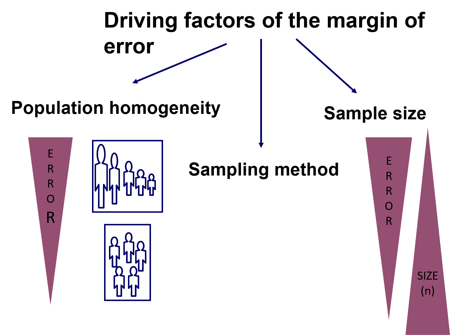
The margin of error will depend, basically on three driving factors:
- How homogenous the data are in the population: the more heterogenous, all other things being equal, the larger the margin of error.
- The sample size: the smaller the size, all other things being equal, the larger the margin of error.
- The sampling technique: depending on the characteristics of your data.
We cannot do much about (a), but there is some room for acting on points (b) and (c). Regarding point (c) about the sampling tecchnique applied, it is important to note that there are a high variey of available sampling techniques that we could apply. The diagram below shows this variety in visual terms:
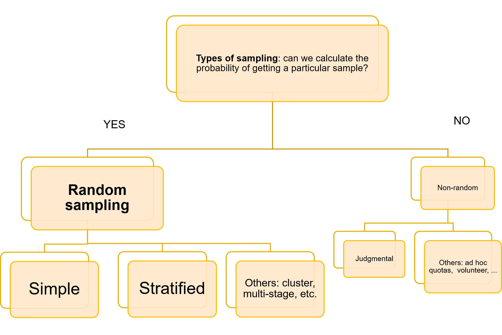
We can only control for the margin of error of our conclusions if we work with random samples and the most frequently random sampling techniques are the simple random sample and the stratified random sampling.
Sampling techniques
Simple random sampling Click to read
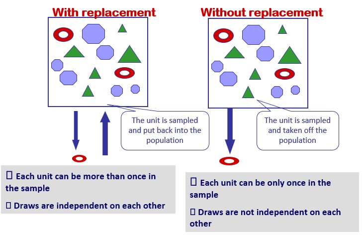
Simple random sampling is the most elemental sampling technique that relies on random selection of the observations surveyed. It consists on, departing from a listing on the units of the population, selecting randomly n of these units. But even within this simple technique, some specifics of the random selection process can be decided. For example, we can decide if the sampling is going to take place with or without replacement. If the sampling is conducted with replacement, this means that each unit that is randomly selected to be part of the sample is put back into the population after each random selection draw. This obviously implies that one unit can be sampled more than once, but it guarantees that the conditions on which each selection draw take place are equal and constant, and the results of each one of them are independent on each other.
On the contrary, if a simple random sampling without replacement is conducted, each unit is sampled only once, but we cannot guarantee that the conditions are constant along the selection draws. Sampling with and without replacement can produce significantly different results for small populations. They are equivalent only if the populations size (N) is very large.
Stratified sampling Click to read
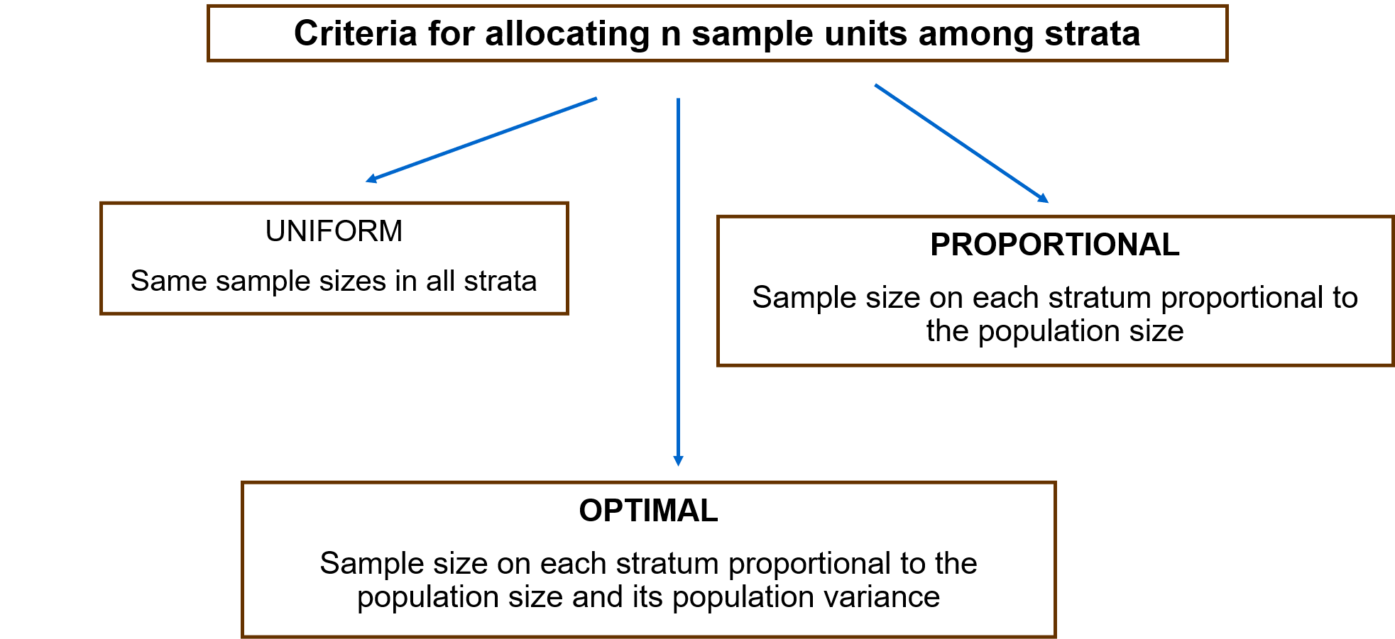
In may occasions, observations are naturally grouped based on characteristics that they share. For example, data on the distribution of wages are grouped depending on the economic sector of the workers, or they gender, or their region of residence. Strata are defined as parts of the population of interest that present a high internal homogeneity, even when there is a large variability between strata. Stratified sampling takes advantage of these grouping of the observations and selects randomly a number of units on each stratum L (nL), such us the total sample size is obtained by summing up the elements sampled on each stratum. There are several criteria for allocating the total sample size across strata, being the most common the following:
- Uniform: same sample size on any stratum
- Proportional: proportion of sample members the same as proportion of population members in each stratum
- Optimal: proportional to the size and heterogeneity (variance) on each stratum
Under the same conditions and with the same requirements of precision and confidence, we can affirm that, generally speaking, stratified sampling requires smaller sample size than simple sampling, but issues related to calculating sample sizes will be detailed in the next point.
Calculating Optimal Sample Sizes
Calculating Optimal Sample Sizes Click to read
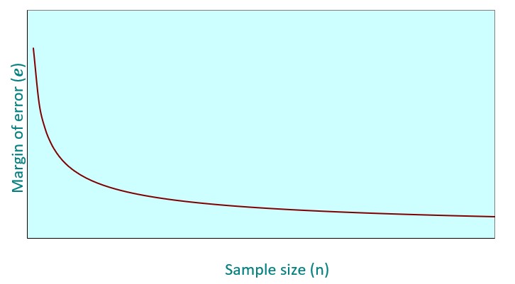
The golden rule in terms of relating the sample size with the precision of our estimates is that the larger the same size, all other things being equal, the smaller the margin of error. However, getting statistical data, even if it is in the form of a sample, can be costly and sometimes we do not have resources to have large samples. As a consequence, there is a compromise solution that sets the optimal (minimum) sample size that we need, given our requirements in terms of precision (margin of error) and confidence of our estimates, and the heterogeneity (variance) of the variable of interest in the population.
|
Rule: the higher the sample size, the more accurate the estimate
|
|
 |
|
Solution for simple sampling Click to read
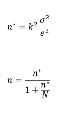
Assume first that we want our sample to estimate a population mean for a continuous variable, and our sample is going to be selected applying simple random sampling. The formulas that we need to apply are the following:
Constant k comes from a normal distribution and gets higher if we increase the desired confidence level and the symbol e stands for the margin of error we are willing to assume. Additionally, we need to make and assumption on the homogeneity of the variable in the population. This implies that we need to impose a realistic value (usually coming from some previous study) on the population variance σ 2.
In these equations, n∗ is the solution for a simple random sampling with replacement, n is the solution for a simple random sampling without replacement and N is the population size. Generally speaking  , and both solutions converge when N is very large. , and both solutions converge when N is very large.
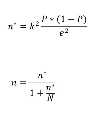
On a similar fashion, if we are interested in estimating the proportion (P) of units in a population that hold a given characteristic, the expressions required to find optimal sample sizes in this sampling technique are:
Again, the constant k comes from a normal distribution and gets higher if we increase the desired confidence level, and the term e stands for the margin of error we are willing to assume. In this case, We need to make and assumption on the value of P*(1-P), which is the variance of a binary (yes/no) variable. The usual solution is to suppose P=1-P=0.5, so P*(1-P)=0.25 takes its maximum value.
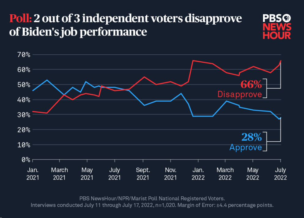
We can illustrate this technique by presenting a practical example on how sample sizes are determined and how applying R can help us on this regard: the Public Broadcasting Service (PBS) in the US regularly estimates the percentage of citizens that approve or disapprove the job of the president. In the case of President Joe Biden, they have been conducting these polls since January 2021. The following chart shows the evolution of their estimates:
In a recent poll along this series, PBS wanted to have estimates with a 99% confidence level, they were willing to have a margin of error of ±4.4% and they assumed the worst-case scenario (usual solution) and suppose that the percentage of people approving (P) is the same as the percentage not approving (1-P). What would be the number of citizens to be sampled with these conditions? The equations displayed above can be implemented in R language to find a solution
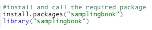
First we need to install and load the required packages:
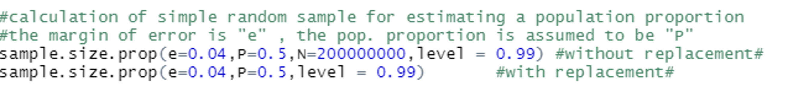
And later, we can find this optimal sample size by calling the function “sample.size.prop” in the package. This function allows for a sampling with or without replacement, although no practical differences will be found between the solution of these two alternatives given the large population size (N) from which the samples are drawn (we can arbitrarily assume that N=200,000,000). The following pieces of code calculate the respective solutions for a sampling without and with replacement:
Which in both cases finds as solution a sample size of approximately 1,000 units.
Solution for stratified sampling Click to read
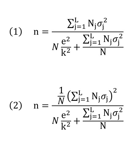
In this point the formulas for calculating sample sizes in the case of stratified sampling are detailed. For the shake of simplicity and clarity, we will focus only on the case of estimating a population mean, and we will offer the two most common solutions, which correspond to the cases of proportional (1) and optimal allocation (2):
As commented above, in both cases the formula corresponds to the estimation of the population mean for a continuous variable with a stratified sampling without replacement. In these expressions Nj stands for the size of stratum j and σj2 for the variance of the variable on this same stratum.
Similarly to the solutions detailed for simple random sampling, we can illustrate how optimal sample sizes are calculated in stratified sampling by presenting a practical example applying R language.
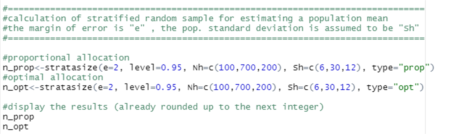
Assume that a charity is conducting a sample survey to study the annual donations made by its members, which are classified in three different groups according to their age with 100, 700 and 200 members each. From a pilot study this charity knows that the respective standard deviations (σj) in the annual donations in each group are €6, €30 and €12. We want to find the minimum sample size required to estimate the mean annual donation, setting a margin of error of €2 and a confidence level of 95%.
The following code lines will calculate the optimal sample size, offering the solutions for the case of a proportional and optimal allocation, by calling the function “stratasize” included in package “samplingbook” in R:
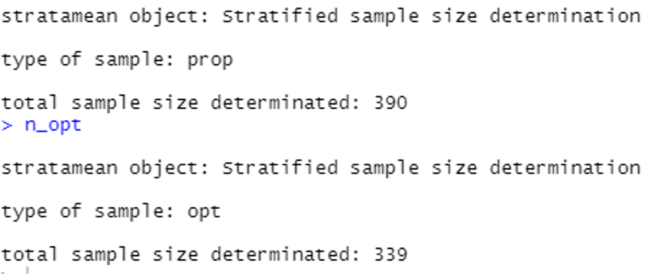
The respective solutions are 390 and 339 units, as detailed below:
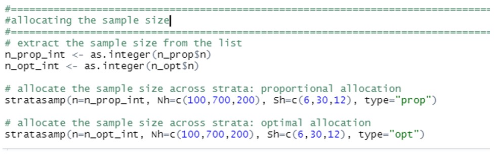
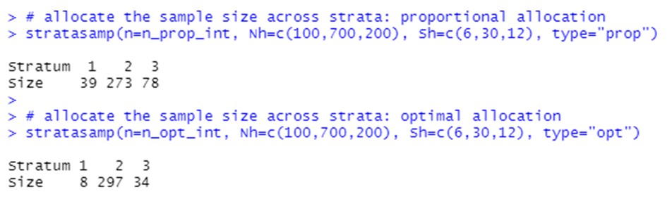
Finally, we can wonder of these two sample sizes will be allocated across strata, This can be done by calling the function “stratasamp” in the same package:
Being the solutions:
|
 Play Audio