DataScience Training
 Play Audio


|
Introduction to machine learning Introduction to machine learning Definitions (Basic) Click to read
 Data Science is an empirical discipline that combines data with various methods, drawn mostly from Statistics and from Machine Learning, in order to solve problems and enable informed decisions. Statistics has been addressed in a separate course, so here we will focus on the field of Machine Learning (ML). There are many buzzwords that are associated with ML – the two most prominent ones are Artificial Intelligence (AI), and Deep Learning (DL). AI is the field of study related to algorithms that can perform tasks normally associated with human “intelligence”. This includes such things as algorithms that can recognize images, or that seem to “understand” text (yes, like chatGPT); that can move around independently (robots, or self-driving cars), or make complex decisions (like whom to give a loan to, or which job applicants to hire). If the method for accomplishing these tasks is to give the machine step-by-step instructions on how to do so, then this is often called “symbolic AI”, or “heuristic AI”. In fact, AI has been around since the 1950s, and until computing technology became more powerful, and data more abundant (around 15-20 years ago), most AI was actually symbolic AI. The increase in available data and computing power has led to the rise in popularity and capability of a second branch of AI: ML – “learning” by example. ML is basically the study of algorithms that can be used to detect patterns in data. In ML, the machine is given the instructions for “how to find a pattern”, as well as many examples; from these examples, it detects a pattern, and uses this pattern to solve “new” problems. Deep Learning is a sub-field of ML. DL is a collection of methods that are based on neural networks, which we will look into more closely later. Types of machine learning Click to read
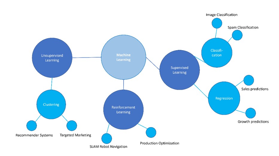
Machine Learning can be further broken down into three classes of algorithms: supervised learning, unsupervised learning, and reinforcement learning. The following figure depicts the different types of machine learning, and provides some examples of application scenarios or use cases for each type.
Figure 1: Types of ML algorithms
Supervised learning Supervised learning algorithms all require labelled data for training, validation, and testing. Labelled datasets are datasets containing feature variables (also known as independent variables, or attributes), and a target variable (also called dependent variable). For example, in a credit-risk detection algorithm, a labelled dataset might include items such as age, gender, account balance, credit rating, and requested loan amount as the attributes; and a target variable – such as whether this person repaid their loan or not. Other examples might be a dataset of images of domestic animals, with labels as to which animal is depicted; or a dataset with features such as a company’s daily stock value over the past 6 months, a yearly average for the past 5 years, and the number of employees, and the target variable would be the company’s stock value on the next day. Depending on the type of target variable, the supervised learning algorithm can be designated as classification, or regression. Generally, when the target variable consists of a finite number of categories, the algorithm is called a classification algorithm. If instead the target variable is a quantitative (or numeric) variable, then the algorithm belongs to the class of regression algorithms. Unsupervised learning Unsupervised learning is used to detect patterns in unlabelled data. Some of the most popular types of unsupervised learning are:
Reinforcement learning (RL) Reinforcement learning is used in order to derive an optimal strategy in situations where the algorithmic agent is required to interact with a given environment, and make a sequence of decisions before the end result is known (i.e. the feedback is not immediate: success vs failure, win vs lose). RL methods are most commonly used in game-playing, or in autonomous driving, and robot mobility. Sometimes a fourth class of algorithms is considered: semi-supervised learning. This is a mixture between supervised and unsupervised learning, and has grown in popularity due to the expense of obtaining labelled data. Often, the nature of the problem at hand, and the type of data that is available, will help you decide which class of machine learning algorithm to use. Are you just trying identify sets of data points with some kind of similarity, without having a clear idea of what these sets should look like? Then you want unsupervised learning. Does your problem involve developing an optimal strategy in a situation where the feedback (success/failure) is not immediate? Then you are looking for a reinforcement learning solution. Or do you have a fixed set of categories, and want to automatically assign new data points to these predetermined classes? Then that’s supervised learning. However, establishing exactly which supervised/unsupervised/reinforcement learning method to choose is a much trickier affair. ML is an empirical science, and you will usually need to try several different algorithms and compare their performance, in order to identify “the best”. For this reason, in the next section, we will describe various ML techniques and their weaknesses and strengths; and in the final section, we consider how to evaluate their performance.
Overview of ML Algorithms Statistics basics [BASIC] Click to read
This section provides an overview of various algorithms that are used in ML. The algorithms range in complexity, from simple algorithms such as decision trees, to the more complex, such as random forests. This section is by no means exhaustive, but should give you a sense of the depth and variety of techniques available in machine learning. Linear Regression is an algorithm used for supervised learning regression problems. Logistic regression is based on the linear regression concepts, but despite the word “regression” in the name, is actually used for classification problems. In fact, if you take a closer look at many concepts and algorithms in ML, you will see that they often boil down to variants of linear or logistic regression. For example, a neuron in a neural network often used to be a simple logistic regression (or something even simpler, such as a piecewise line!) Although they are also part of the ML toolkit, linear and logistic regression have been studied extensively in Statistics, and will not be described further here. See the STATS scriptum. Naive Bayes Classifier [BASIC] Click to read
Naive Bayes is a simple classification algorithm that is often used as a base-line (to compare to other, more complex algorithms) in natural language processing problems, for example. Naïve Bayes uses Bayes’ Theorem to transform the problem of determining the probability of an instance belonging to class Y, given its attributes X = [x1 , …, xN], into the easier problem of evaluating the frequency of attribute xi , given that the instance belongs to class Y. Bayes’ theorem is a simple mathematical formula used for calculating conditional probabilities. The theorem states that:
P ( Y|X) = P (Y) is the probability that event Y occurs, P P (Y|X) is the probability that Y occurs given that X occurs (the conditional probability of Y given X). Another way to write Bayes’ Theorem is P Why is this useful? Because the relative frequencies of X given Y in the training data can be used to determining P (X|Y).
It can deliver good results when
Naive Bayes comes in different variants:
Decision Trees [INTERMEDIATE] Click to read
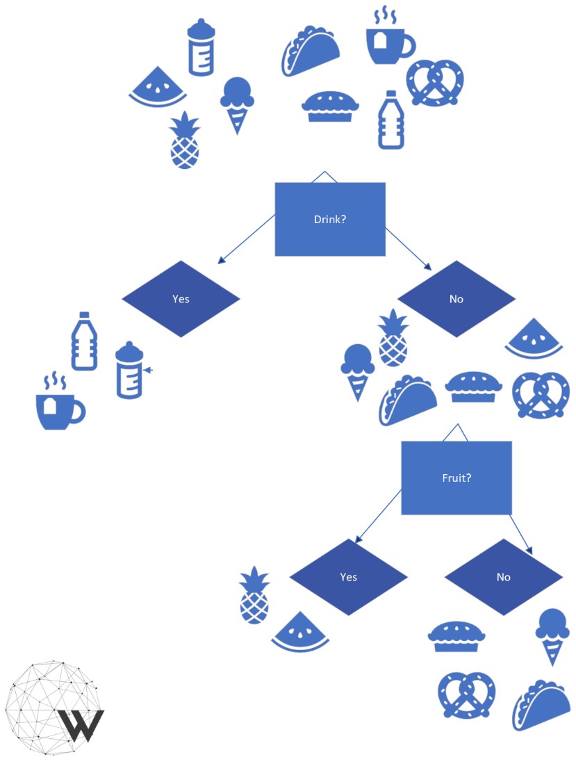
A decision tree is a supervised learning algorithm that can be used for classification and regression modelling. Decision trees are both a way of representing information, and an algorithm for detecting patterns in data. In fact, a decision tree algorithm outputs the information it has “learned” from the training data in the form of a decision tree. So what does a decision tree look like?
Figure 2: Classification Trees A tree whose leaves are classes, or categories, is called a Classification Tree. When the leaves are functions (most often numeric constants, or else lines), this would be a Regression Tree. Decision tree algorithms are constructed using methods from information theory, and tries to construct a tree according to the principle of “most information gained” at every step. Commonly, the number of branches, and the depth of the tree, are choices that the data scientist has to make – a bit of experimentation with different values is often necessary. It is also good to keep in mind that having trees with a larger number of branches and of a greater depth provides more flexibility, but this has to be weighed carefully against the increased chances of overfitting, and the fact that trees with fewer branches and of lower depth are eminently more understandable. Random (decision) Forests [INTERMEDIATE] Click to read
A random forest is a collection of many decision trees that operate as an ensemble. Random forests are a special kind of “ensemble learning” – a class of methods that combine (usually simple) models to improve predictive accuracy through diversity. Random forests consist of multiple randomly chosen decision trees, and combine their predictions. They vary in the number of trees they contain, and the depth of each tree. Random forests are often seen as a combination of the explainability of decision trees, and the power and increased accuracy of more complex methods. Random forests, and other tree-based ensemble methods such as gradient boosting, are still quite popular, and can achieve state-of-the-art results (yes, it doesn’t always have to be a neural network). Hierarchical Clustering [BASIC] Click to read
Clustering is a broad set of techniques in unsupervised learning. The goal is to detect structure and similarities in the data: to find a grouping of the examples in the dataset so that the examples in one group are somehow similar to each other, and different from the examples in other groups. A popular application would be consumer profiling: identifying “types” of consumers, so that ads can be more targeted. Hierarchical clustering and K-means clustering are two of the most prominent clustering techniques. Hierarchical clustering produces a tree-like structure (in this case usually referred to as a dendrogram), which starts at a top node containing the entire dataset, and recursively, at every node, branching into smaller dendrograms, where “similar” items go into the same branch. This kind of clustering provides different levels of granularity: looking towards the top of the dendrogram we have a broader concept of “similar”, and as we progress down towards the bottom, the differences between branches are more subtle. K-Means Clustering [BASIC] Click to read
Whereas hierarchical clustering does not require any information on the number of groups, or clusters, to split the data into, K-means clustering does. In fact, in K-means clustering, the dataset is split into K distinct groups. It is often not a priori clear how many groups a dataset needs to be divided into. For this reason, part of your job as a data scientist would be to experiment with a few different values of K, to find the “best” one. The K-means algorithm assumes each instance in the dataset is a point in a vector space with a given distance function (usually Euclidean). It starts by randomly assigning each instance in the dataset to exactly one of K clusters, and then computes a centroid, or mean, for each cluster. It then goes through and reassigns each point to the cluster whose centroid is closest; cluster means are re-computed, and points reassigned again. This process continues until the reassignment process does not change the cluster membership of any of the points in the dataset. A word of caution: the clusters are not robust, and in particular, the initial random assignments of points to clusters have a strong influence on the results. You should run the K-means algorithm several times, and then choose the best clustering. And how is it possible to determine which is best? If we already have a notion of distance, then for each cluster, we can compute how much variation there is between points in that cluster. Take the sum over all K clusters: If the groups make sense, and each cluster contains points that are similar to each other, then we expect the sum to be small – so we choose the clustering with the lowest sum. Neural networks Click to read
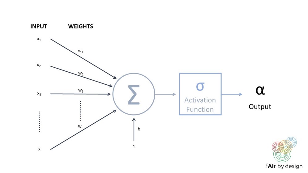
A neural network consists of a series of interconnected units (so-called "neurons"), like the one depicted in the figure below. Each neuron takes in multiple inputs, assigns each input a weight, then combines and runs them through an activation function, to produce one output. The sigmoid function is often used as an activation function – which means the neuron is acting like a logistic regression! But the most popular activation function currently being used is even simpler – it is called a rectified linear unit (ReLU), and takes the value f(x) = x when the input x is positive, and f(x) = 0 when x is negative.
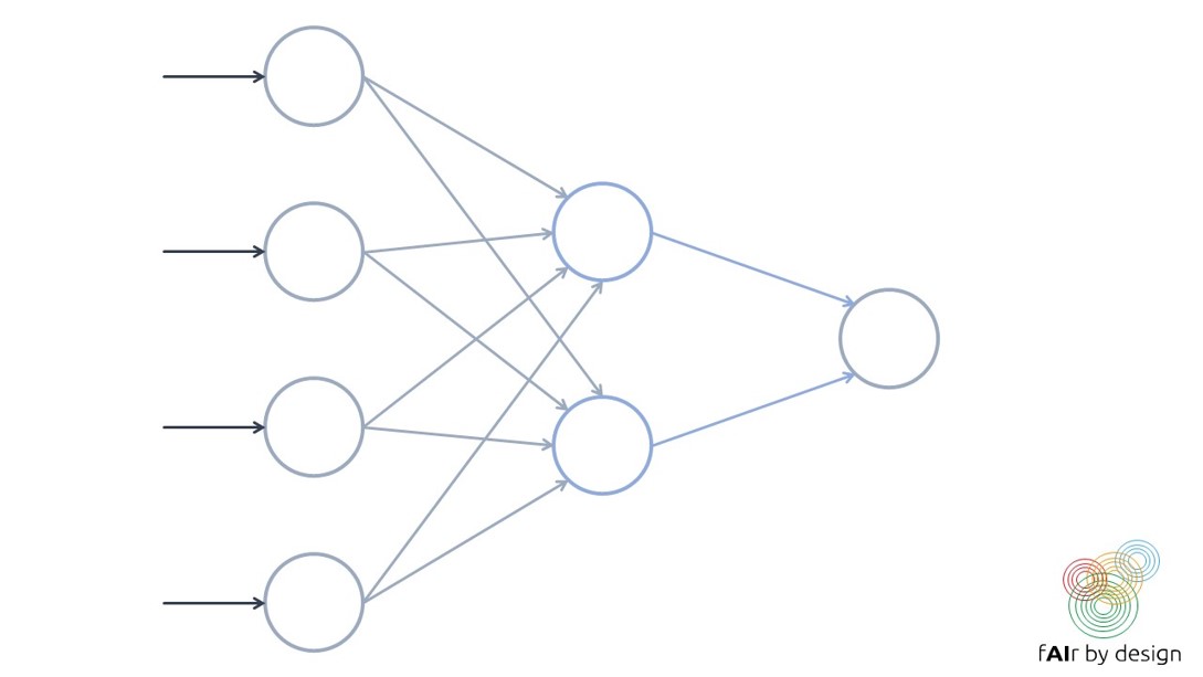
A neural network is formed by organizing these so-called neurons into layers. Training a neural network means trying to establish the values for the network weights that minimize prediction error on the training data (as measured by a given loss function).
As you can see, the building blocks of a neural network are quite simple. What makes them so complex is the sheer number of “neurons” they have, the number of layers, and the different ways the neurons can connect to each other.
Evaluating Performance Accuracy and Co Click to read
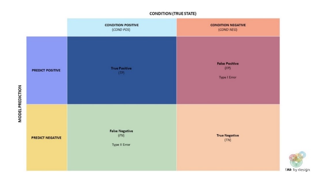
There are many metrics that can be used for measuring the performance of a trained model. Which one to use depends on the type of model (supervised, unsupervised, or reinforcement learning; classification vs regression), and on the context of use. We will focus on supervised learning. In the supervised learning setting, datasets need to be split into training, validation, and test sets. The test sets should never be seen in training or in validation: they should be “locked away”, and pulled out only at the very end, in order to test how the model performs on completely new data. Only if this is done, and only if the test data is representative of the model’s intended use context, can the model performance on test data be considered an indication of how it will perform “live”. This also means that different usage contexts require different test sets! Validation data is used to help choose a “best” model. For example, say you have a decision tree classifier, where you are trying to decide what is the best “depth”, and you also want to compare with a Naïve Bayes classifier: use the performance on the validation data set to make the comparison. One important issue bears repeating: if a dataset has been used for validation, it cannot be used as a test set. With this principle in mind, you can, however, use the validation data for more than one validation or model comparison. Finally, the training data set is the dataset that is used to train the model. Ideally, also the validation data should be completely separate from the training data. However, in circumstances where data is scarce, it is possible to use bootstrapping or cross-validation (see below) to use the training data set for both model training, and model validation. Once a test or validation set is established, we also need to know how to measure the performance of the model. Remember that for a supervised algorithm, the examples in the dataset all have the “correct” target value, which can be compared with the model’s predicted value.
However, these are not always the «best» metrics to use, as the examples below will show. Binary classifiers are classification systems where there are only two possible target classes: let's call them POSITIVE and NEGATIVE. We will examine different performance metrics for these, and why in certain circumstances, they are preferable to accuracy. Lets start with a commonly used tool to help understand the performance of a binary classifier: the confusion matrix.
Using the terminology from the confusion matrix, we can write down a formula for accuracy: Accuracy = (TP + TN)/(TP + TN + FP + FN) When would you want to use a metric other than accuracy?
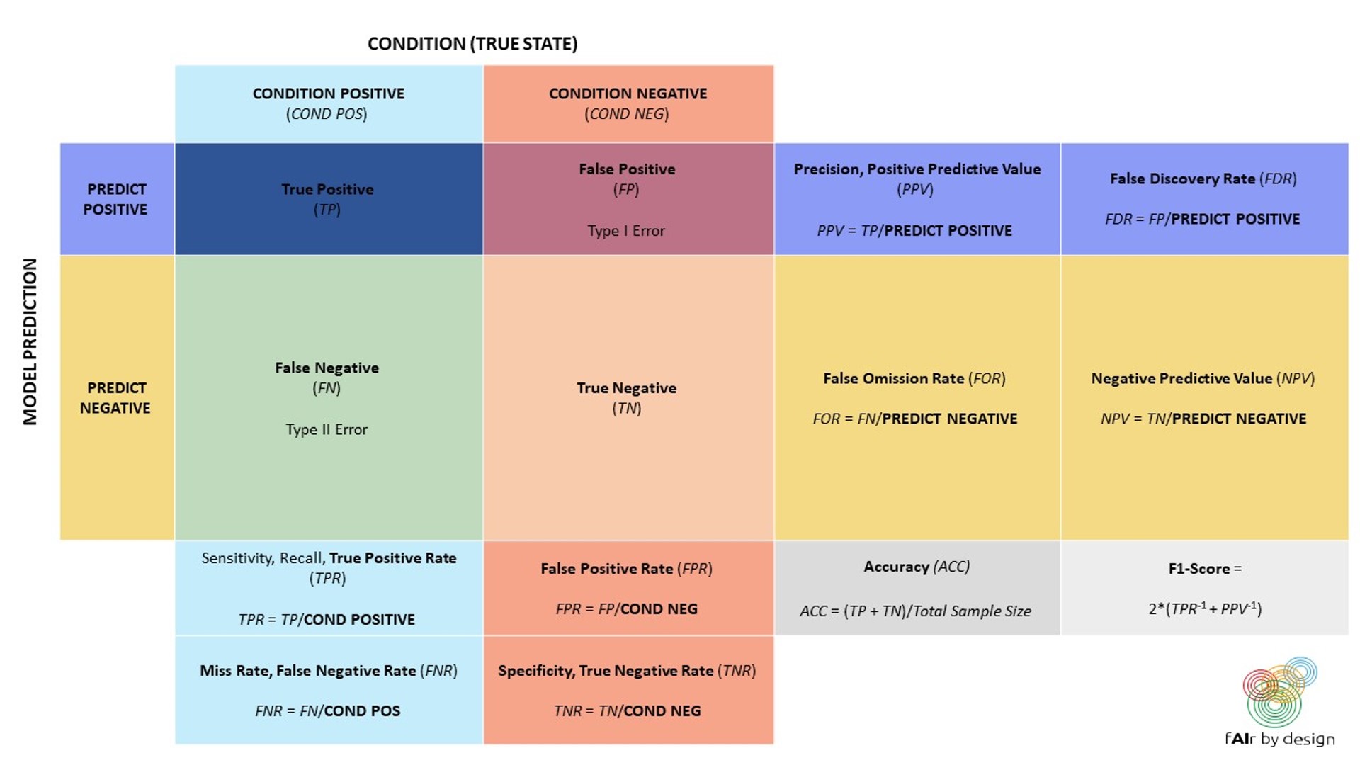
A more expanded version of the confusion matrix, shown below, can help with the choice of metric:
So, if you need to identify all POSITIVE elements, then your model should have a high sensitivity, or True Positive Rate (TPR). If instead you want to avoid false POSITIVES, then your model should minimize the False Positive Rate (FPR) – which, examining the confusion matrix, is equivalent to maximizing the specificity, or the True Negative Rate. Even when it may be clear that you have the correct metric (or metrics – you can try to optimize more than one, or find a balance between several), what is the point where you say "this is good enough”, and decide to use the model? There is no textbook answer to this question – it depends on the context. As an example, lets consider a „real-life“ application: automated hate speech detection on social media. According to data obtained in Amnesty International Italy‘s „Barometro dell‘Odio“ project (see the data4good slides), hate speech makes up about 1% of online political content. Since the target class is so imbalanced, accuracy is not the best choice of metric. Suppose you developed a hate speech model that was optimized for high TPR and low FPR: it achieves 99% TPR and 1% FPR. Then for every 100 comments that the model classifies as hate speech, how many can be expected to actually be neutral comments? Try to figure it out yourself before reading the excel sheet below!
You can use the above spreadsheet to play around with different TPRs, FPRs, and prevalences. This should give you a feel for the importance, not just of metrics based on your test set, but also for trying to understand the impact of the model in its context of use. For example: knowing what you do about the percentage of neutral comments it would flag as hate speech – would you recommend that the model be used to classify and automatically censor hate speech comments?
Bootstrapping Click to read
Bootstrapping is based on doing a Random Sampling with Replacement (that means, one takes the vase with colored balls, so common in probability texts, that one randomly pulls out a ball, notes the color, and throws the ball back into the vase) on the training data. This means that the same observation can be drawn several times, while other observations may not be drawn at all. This statistical fact is exploited: samples are drawn from the training data as often as necessary until a new training data set of the same size is obtained. Those observations that were never drawn in this procedure are put into the validation data set. The validation results are used to compare the different algorithms Cross-validation Click to read
There are different ways to perform cross-validation, but we focus on n-fold cross-validation, and set n = 5 for simplicity. The training dataset is divided, by random sampling, into 5, roughly equal sized subgroups.
Once the validation is complete and a „best“ model has been selected, it can be re-trained on the entire dataset.
Other considerations Click to read
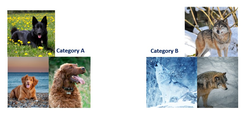
There are situations where these measures of performance are not enough. Consider the following example, in which an image classifier has detected a pattern and can classify images as “dog” vs. “wolf”.
DOG WOLF How do you think it will classify these next two images?
The image on the left was classified as “dog”. The one on the right as “wolf”.
Why? Because the model actually wasn’t detecting dog vs. wolf, but rather snow vs. no snow. This example is inspired by the article “Why should I trust you?” [1]. As long as the model is too complex for us to understand which patterns it has learned, and why a particular prediction was made, it is difficult for us to detect mistakes. There are situations where it can be much more important to be able to understand what patterns the model has learned, than to gain a few extra percentage points in accuracy. Beyond explainability, other possible requirements on the model could be security (against hackers, or data poisoners for example), privacy (if the algorithm needs to process sensitive data), or non-discrimination (see the data 4 good slides). There are many criteria that combine to create the “best” model – accuracy may be just one of them.
Further Reading Click to read
This script has just gotten you started on you ML journey. If you are curious to learn more and try out some problems, we highly recommend the textbook “An Introduction to Statistical Learning” [2]. |


Keywords
Keywords (meta tag) Machine Learning, supervised learning, classification, regression, AI, artificial intelligence, naive bayes, decision tre&#
Objectives/goals:- Learn about AI, machine learning, deep learning, and how they relate to data science
- Learn about different algorithms used in machine learning, including:
- Naive bayes
- Decision trees
- Random forests
- Neural networks
Brief overview of how the performance of machine learning algorithms can be evaluated
This script provides definitions of the fundamental concepts in machine learning, as well as descriptions of the main methods used, including some specific examples and applications. You can choose to read the script at a superficial level, to gain a basic grasp of the field, or read the more in-depth descriptions, in particular the methods section, to obtain an intermediate-level understanding of machine learning.
Statistics and Machine Learning provide the main tools for your work as a data scientist. Understanding the various machine learning methods - how they work, what their main advantages are, and how to evaluate their performance on a given task - can help you make better decisions about when to use them and will make you a more versatile data science expert.
[1] Ribeiro, M. et al, "Why Should I Trust You?": Explaining the Predictions of Any Classifier. Available on arxiv: https://arxiv.org/abs/1602.04938
[2] James, G. et al, An Introduction to Statistical Learning, 2nd ed., 2021. Available at https://www.statlearning.com/
Related training material