DataScience Training


Linear discriminant analysis
Feedback form    |       Play Audio    |   Download:    |   


Linear discriminant analysis

Introduction

Motivation by an illustrative example Click to read  

Suppose that we have a sample of individuals, and we observe the transportation mode (by car, by public transport or by walking) they usually take to move within a city. We know that the choice of the transportation mode is partially influenced by their economic status, and we observe data on their age in years and their household annual income, together with the chosen mean of transportation:

We want to know how these two covariates help to classify (i.e., discriminate) the individuals by assigning them to a specific category of transportation mode. We can see that there is not perfect classification: individuals with high income tend to use cars more frequently, but there is great overlap of “walking” and “public transport” categories for those with lower incomes. And there is a larger overlapping among categories regarding their distribution by age: older individuals do not walk, but at younger values age is not a good predictor of transportation mode. This is the typical problem that LDA addresses.


LDA for classification

Formulation Click to read  

ØLDA functions can be recovered to help with the classification of the data based on a matrix of covariates X
 
ØSimilar to Principal Component Analysis (PCA), LDA functions aim at finding a linear combination of the original data as:
 
 
Øwhere the between-class variance (B)  is maximized relative to the within-class variance (W), which can be approached as a generalized eigenvalue problem.
ØDiscriminant coordinates are obtained from the eigenvectors of 


An example Click to read  

As an illustrative example, we solve the classification problem of transportation mode basing on age and income by LDA in R. This can be easily done by the “lda” function within the “mass” library. For all the analysis presented here, we will need to install and load the following R pakages:


The data studied comes in a csv file (called “trasnpor_example”), which can be easily imported to R by runing this piece of code:

In ordser to have a first impresion of the data, we can plot the sample in the form of a scatter plot as:

The code lines above produces the scatterplot shown in the introductory section of thid document. Alternatively, we could plot the data as a series of histograms as:

By running any of these two lines, we can have in a glimpse an idea on how transportation mode distribute across values og age and income. For example:

Obtaining:

Or: 

LDA is conducted by simply running:

The typical output shows the initial means by group, the coefficients in the LD projections and the proportion of the between variance (trace) that each LD coordinate explains:

In our example, the first LD coordinate is positively correlated with income and negatively with age, and contains almost 90% of the inter-class variability. The second LD function shows positive but weaker correlation with both variables, and only accounts for approximately 10% of the between variability.

The new coordinates are produced projecting the original data points with the LDA coefficients by the expression ������. In these new coordinates, observations are more clearly separated across groups. In our example, we have two LD coordinates for each individual, given their age and income. The coordinates corresponding to the first LD function have the larger discriminant power. We can easily see this discriminant power by plotting in R an histogram, now putting the first LD coordinates in the horizontal axis:


Obtaining: 

This plot shows how the amount of overlapping diminishes considerably. In other words, the first LD coordinate (remember that it is a “composite” that correlates negatively with age and positively with income) adequately discriminates among the transportation categories.


Predictive LDA

The procedure Click to read  

LDA can be used not only for (descriptive) classification purposes, but also with the objective of predicting class membership. For example, suppose that we have data of the age and annual household income for an (in-sample or out-of-sample) individual, and we’d like to predict the transportation mode that this person is most likely to use. LDA can be helpful in providing us with a prediction, in a similar fashion to multinominal logit or probit models.

For this predictive purpose, some assumptions are required:

  • groups are multivariate normal
  • equal variances-covariances across groups

The formulation of predicitive LDA is related to the formulation of Bayes tehorem for updating probabilities: Let g be the number of groups and qi the prior probability (usually observed relative frequencies) for group i. Let X be a vector of observations of covariates for one individual.The (posterior) probability of belonging to group Gi conditional on X, P(Gi |X), can be expressed as:

This is a Bayesian approach that updates the prior probabilities q_i basing on the conditional probabilities P(X|Gi). Under the normality assumptions:

where |W| is the determinant of the within-class variance matrix and Di  is   . Plugging the expression of in the formula for , we have:


An example with R Click to read  

The LDA routine in R can produce posterior probabilities basing on the assumptions and the formulation detailed before. The LDA functions allows for predicting the most likely class membership for any individual, given a vector of covariates (age and household income in the example).

As an illustration, the table displayed below shows the predicted probabilities for each group for a subset of individuals in the sample. The priors qi are assumed to be identical for each one of the three transportation modes ().

The predicted class corresponds to the highest  for each individual. They are calculated by applying the following routine in Rstudio:

In most of cases, LDA correctly predicts the group to which each individual belongs. There are some cases, however, for which LDA does not predict correctly. These cases correspond to the overlapping observations that still remain in the LDA classification


Keywords

discriminant analysis, classification, R, Bayesian analysis

Objectives/goals:

The objective of this module is to introduce and explain the basics of Linear Discriminant Analysis (LDA).


At the end of this module you will be able to:


  • Identify situations on which LDA can be useful

  • Calculate LDA functions


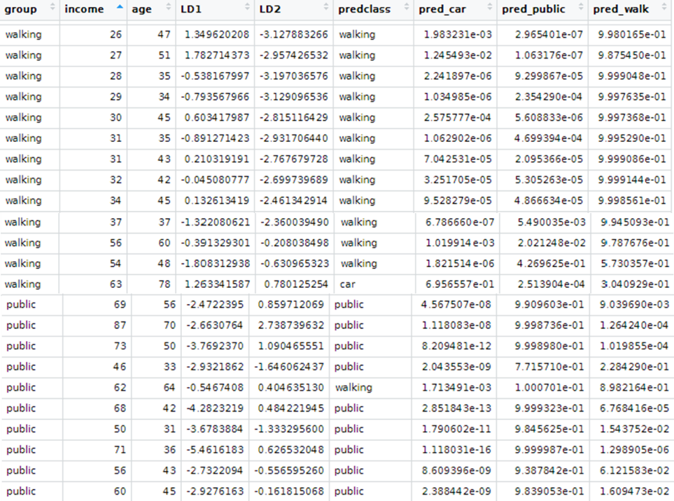
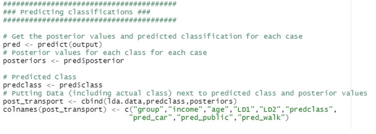
Interpret the results produced by descriptive and predictive LDA


Description:

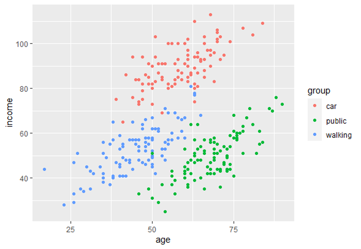
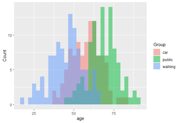
In this training module you will  be introduced to the use of Linear Discriminant Analysis (LDA). LDA is as a method for finding linear combinations of variables that best separates observations into groups or classes, and it was originally developed by Fisher (1936).

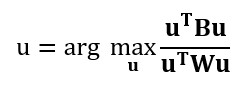
This method maximizes the ratio of between-class variance to the within-class variance in any particular data set. By doing this, the between-groups variability is maximized, which results in maximal separability.

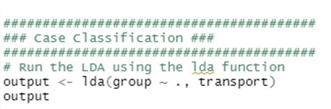
LDA can be used with purely classification purposes, but also with predictive objectives.

Bibliography

Boedeker, P., & Kearns, N. T. (2019). Linear discriminant analysis for prediction of group membership: A user-friendly primer. Advances in Methods and Practices in Psychological Science, 2, 250-263.


Related training material

Partners

Università del Salento
Demostene Centro Studi
IHF
IWS
Universidad de Oviedo
ASE
WAI