DataScience Training
 Play Audio


|
Introduction to RStudio software Introduction Introduction Click to read
 A brief history ●Project R was born in the statistics department of the University of Auckland, New Zealand;
●The founders of the project are Robert Gentleman and Ross Ihaka, now associate professors;
●The project started in 1991, but the first release was in 1996;
●R software is now considered the most powerful statistical computing language in the world;
The Computing Environment
●Cross-platform (Windows, MacOS, Linux);
●Open-source (software, manuals, reference cards, all downloadable from the www.r-project.org website);
●It has numerous integrated tools for data analysis;
●Allows you to implement matrix calculus;
●Easily manipulated and useful for data storage;
●The term environment is intended to distinguish R as a fully planned and coherent system, rather than a collection of extremely specific and inflexible tools.
Statistical Analysis Techniques
Most of the statistical techniques, from the most classic to the most recent, have been implemented in the R environment. Only some of these are integrated into the basic environment, many others are provided in the form of packages, through the family of websites called CRAN (Comprehensive R Archive Network). Community ⮚A community of over 2 million users and developers provides time and technical expertise to maintain, support and develop the R language and environment, tools and infrastructure.
⮚At the heart of the community, the R Core group, of about 20 members, takes care of the maintenance and guides the evolution of R.
⮚The official public structure is provided by the R foundation, a non-profit organization that ensures the financial stability of R-project and administers the copyright of the software and documentation.
Software R How to install R software Click to read
●From the site https://www.r-project.org/
●Click Download R
●Choose the CRAN you want (the physical place from which to download the software)
●Choose the operating system on which to download the program (Windows, Linux, MacO)
●Click install R for the first time
●Start the download
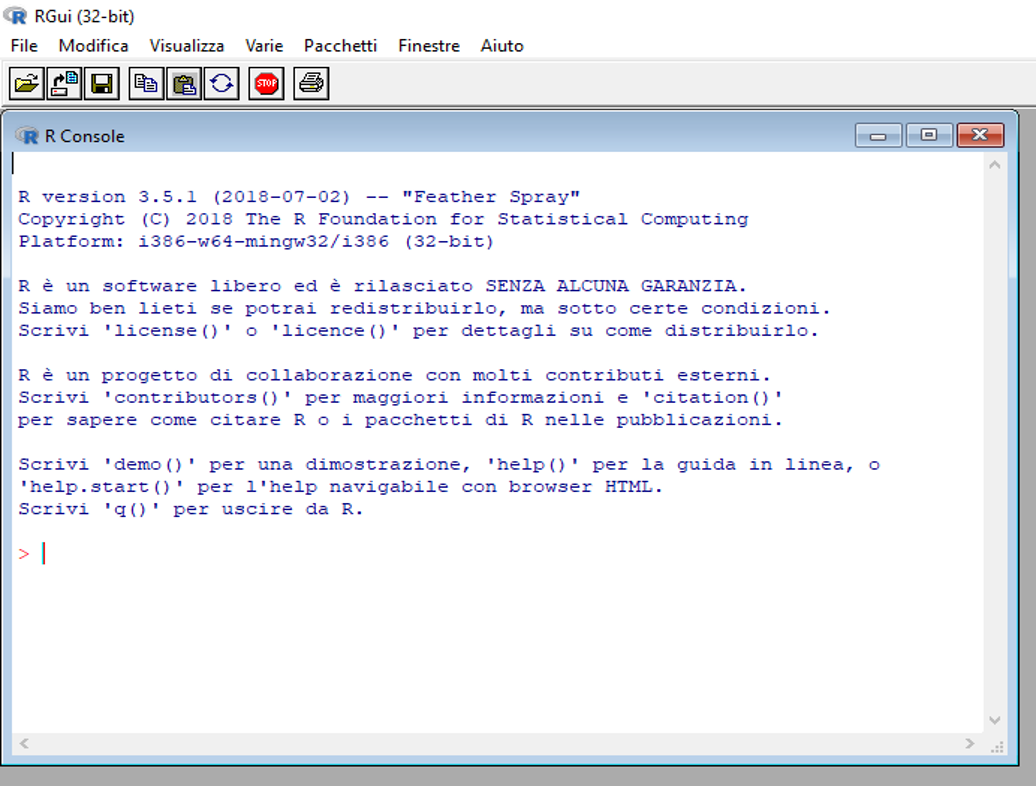
 What R looks like Click to read
RStudio Let's explore RStudio Click to read
⮚The most commonly used and most accessible interface is RStudio, downloadable from the https://www.rstudio.com/
⮚RStudio uses a user-friendly interface to facilitate its use;
⮚Click on Download (RStudio);
⮚Choose the free version;
⮚Start the download;
⮚Integrated Development Environment (IDE) for R
⮚The RStudio working environment consists of 4 windows:
Code window (write//execute scripts) 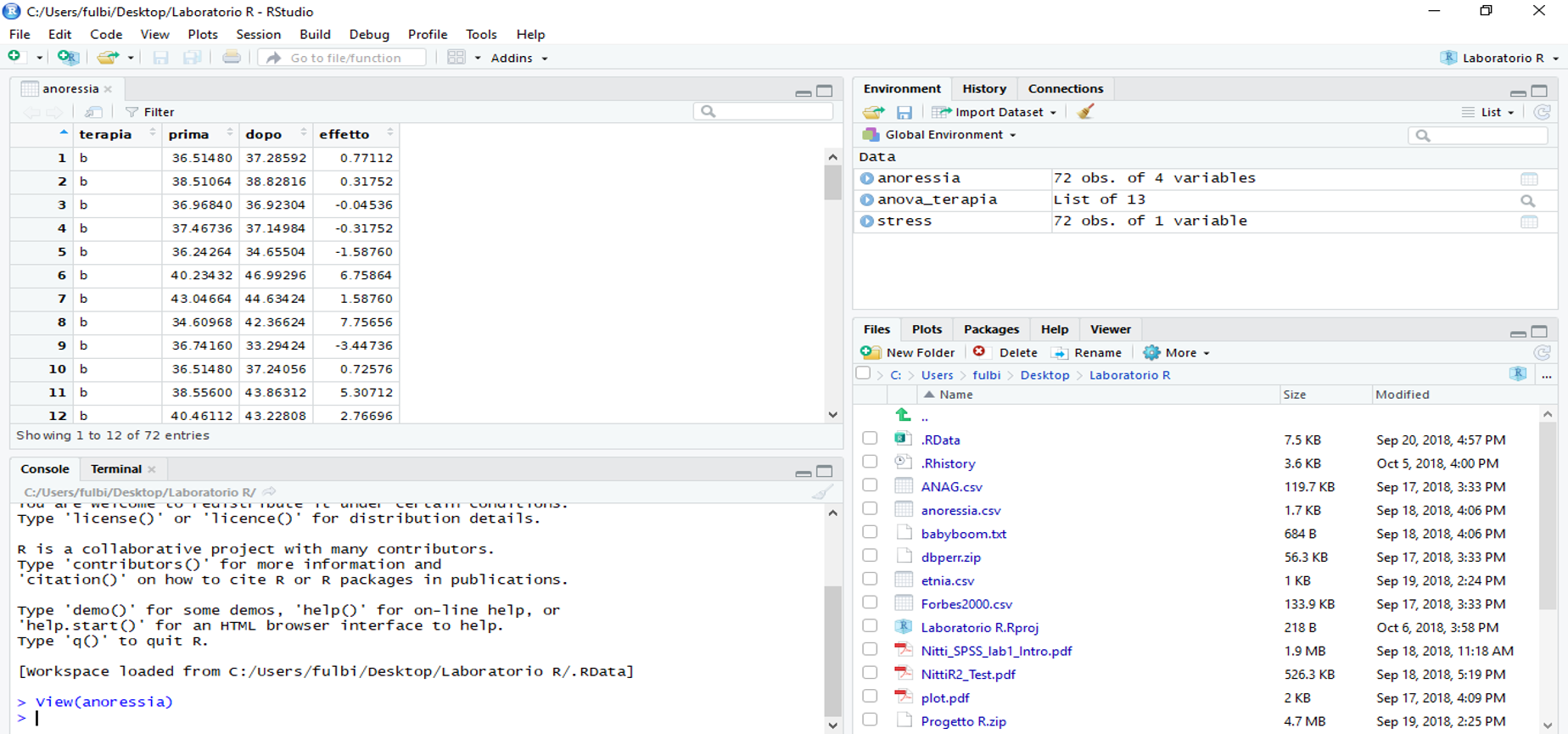 Multi Tab Window
⮚Packages: allows you to download packages that allow you to perform statistical analysis, such as Analysis in Main Components.
Example: click Install and install the ggplot2 package ⮚Help: allows you to have the description of the package.
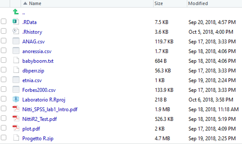
Example: Type ggplot2 ⮚Files: allows you to quickly access saved files after creating an R project
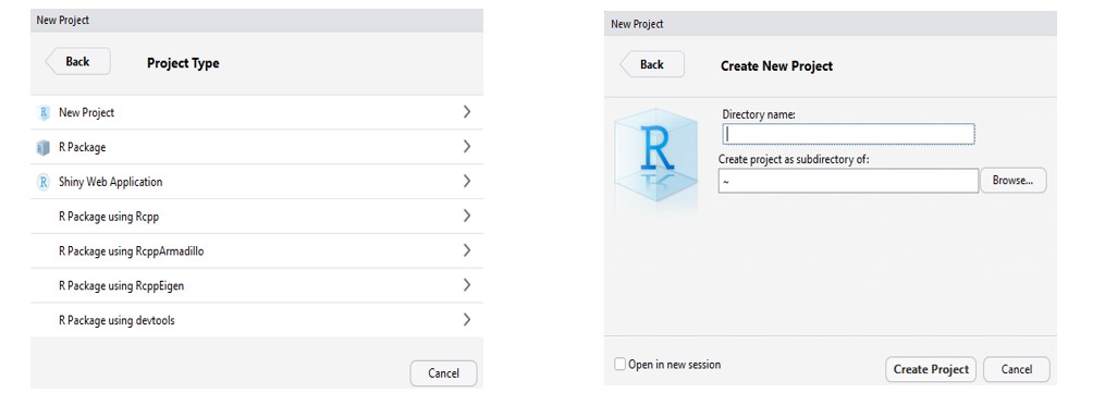
 Creating a Project Click to read
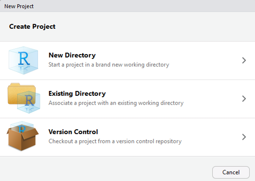
⮚With RStudio you can create a project in order to define the working directory, have all the data, packages and codes inside.
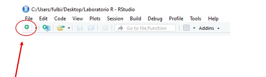
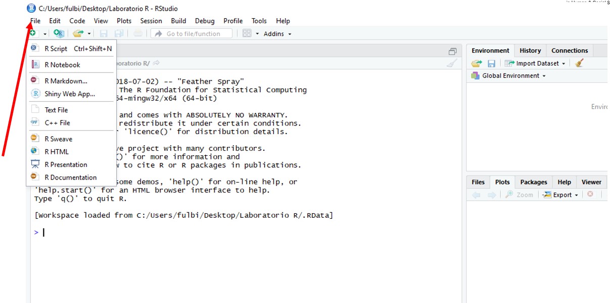
⮚To create a new project, go to the menu at the top left and select File -> New Project
  ⮚Getting Started: Loading Data
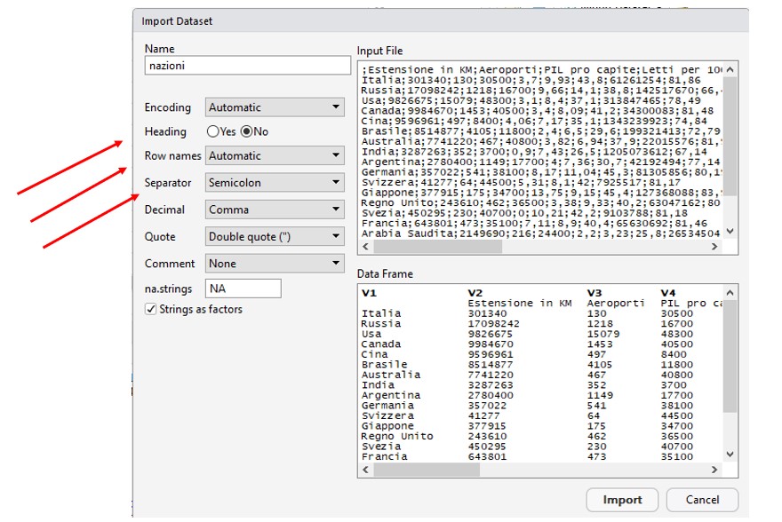
⮚R can read different types of data (TXT, CSV, XLS, XLSX, SPSS, STATA), but the simplest and most immediate way is the CSV format (Comma Separated Value).
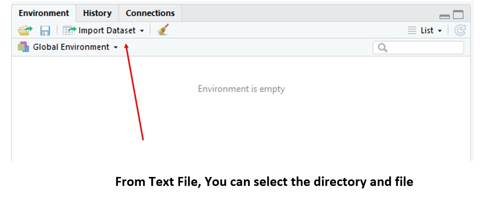
⮚To upload a CSV file select Environment from the menu on the top right -> Import Dataset -> From Text File, Then select the directory and file.
R Notebook & R Script Click to read
⮚They allow you to keep track of the codes and analyzes carried out within the R project and save them on the PC for further consultations.
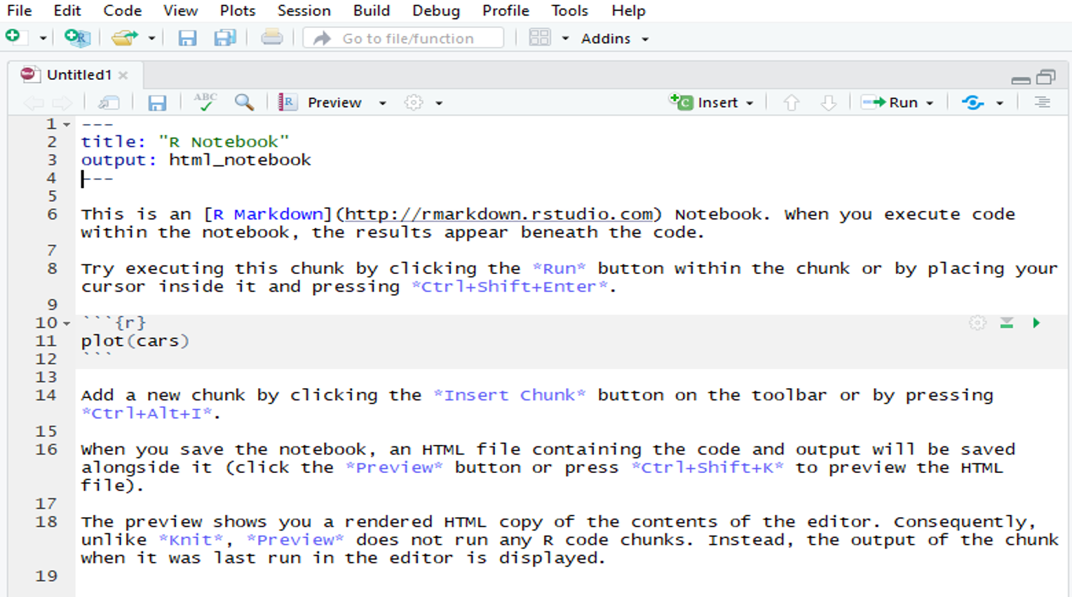
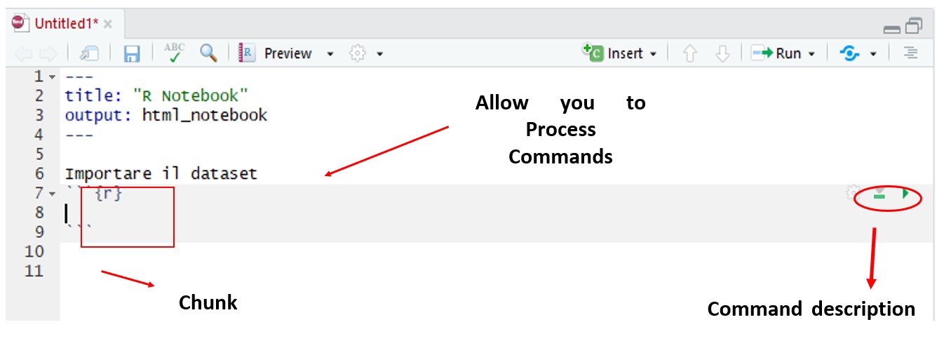
R Notebook Allows you to create a report of a project by entering all the steps, operations and graphs created.
R Notebook: The commands must be inserted inside special chunk (ALT + CTRL + I), the descriptions out
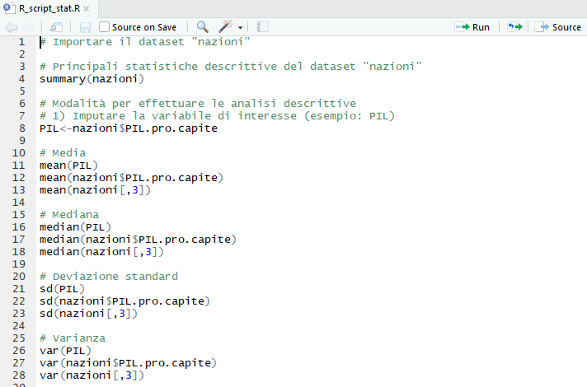
R Script:
Create a file where to insert all the codes useful for the appropriate analysis
⮚Codes can be selected all together and processed simultaneously
Loading a Dataset Click to read
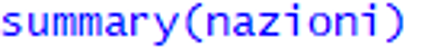
Descriptive Statistics "Summary" Click to read
A first exploration of the distribution of the variables contained in the countries dataset is obtained through the summary command, which must be inserted in the window called Console. summary(name dataset / or name variable)
Other Descriptive Statistics You can assign a name to each column of interest: The main synthesis indices for quantitative variables are: ⮚Media: mean(PIL) or mean(nazioni$PIL.pro.capite) or mean(nazioni[,3])
⮚Varianza: var(PIL) or var(nazioni$PIL.pro.capite) or var(nazioni[,3])
⮚SQM (Standard deviation): sd(PIL) or (nazioni$PIL.pro.capite) or sd(nazioni[,3])
Graphs in R (Plot) Click to read
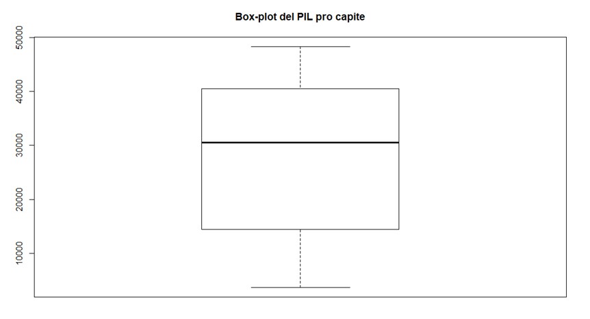
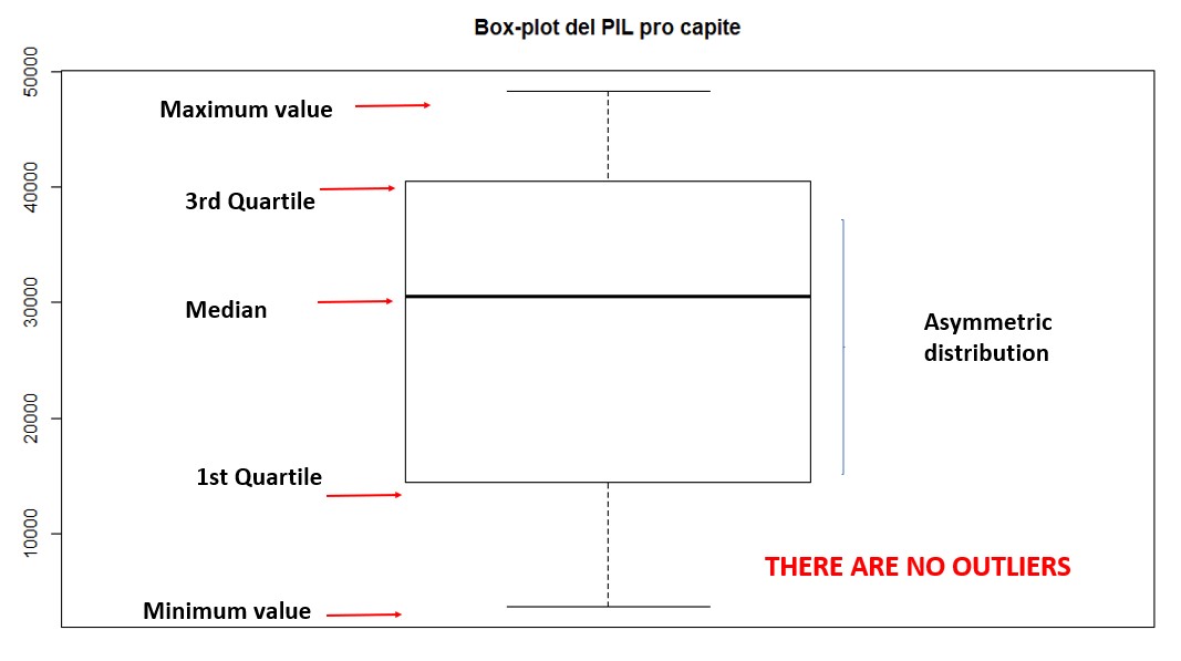
BOX-PLOT: The box-plot describes a quantitative variable through the graphical representation of the minimum, maximum, quartiles and median. ⮚boxplot(nazioni$PIL.pro.capite, main = "Box-Plot del PIL pro capite")
or ⮚boxplot (nazioni[,4], main = "Box-Plot del PIL pro capite")
or ⮚boxplot(PIL, main = "Box-plot del PIL pro capite")
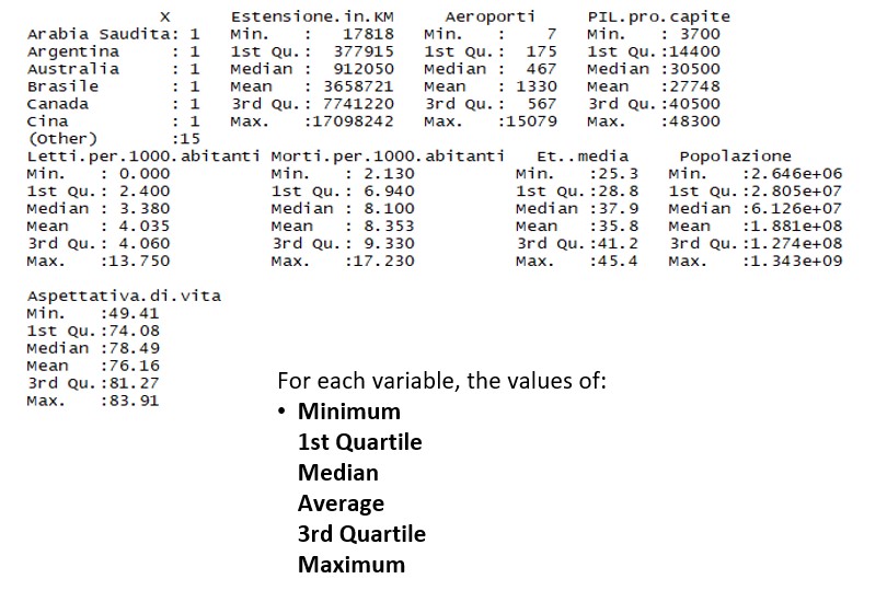
  SCATTER DIAGRAM:
⮚Performing an exploratory analysis on the type of relationship between two variables
⮚Example from the dataset: analyze the relationship between average age and life expectancy. Is there a relationship
⮚1) Name variables of interest
eta<-nazioni$Et..media asp<-nazioni$Aspettativa.di.vita The command to prepare the scatterplot is: plot(asp, eta, xlab="Aspettativa di vita", ylab="Età media")
SCATTER DIAGRAM: What can you say?
From the scatterplot there appears to be a relationship between the variables Life expectancy and Average age. Specifically, as the average age increases, life expectancy increases.
Correlation analysis:
MODERATE CORRELATION QUALITATIVE ⮚Load datasets ANAG
⮚Name the column Gender -> sesso<-ANAG$Sesso
⮚For qualitative variables, the first description concerns the frequency distribution analysis.
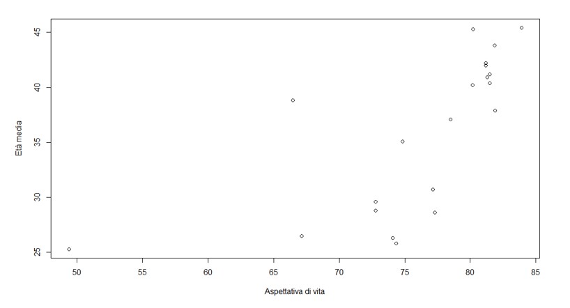
Create the frequency distribution for the variable «sesso» -> table(sesso) 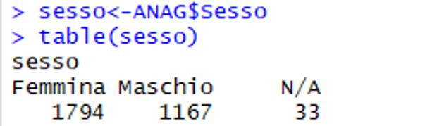 PIE CHART
⮚A mode of graphical representation of the distribution of qualitative characters is the piechart, whose segments are proportional to the frequencies of each category.
x<-table(sesso) ⮚Pie chart without percentages:
pie(x, main = "Grafico a torta sul sesso")
PIE CHART WITHOUT PERCENTAGES
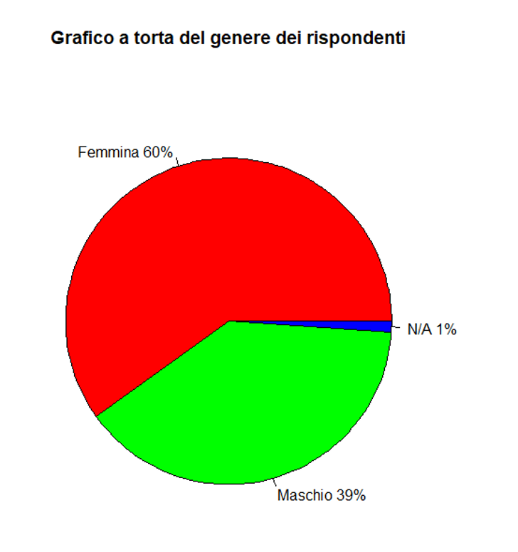
PIE CHART WITH PERCENTAGES labels <- c("Femmina", "Maschio", "N/A") #ADD LABELS n<-lenght(ANAG) #IMPUTATION OF SAMPLE NUMBERS pct <- round(x/n*100) #CALCULATION OF PERCENTAGES lbls <- paste(labels, pct) # ADD PERCENTAGES TO LABELS
lbls <- paste(lbls,"%",sep="") # ADDS THE SIMBOL % TO LABELS pie(x,labels = lbls, col=rainbow(length(lbls)),main= "Grafico a torta del genere dei rispondenti")
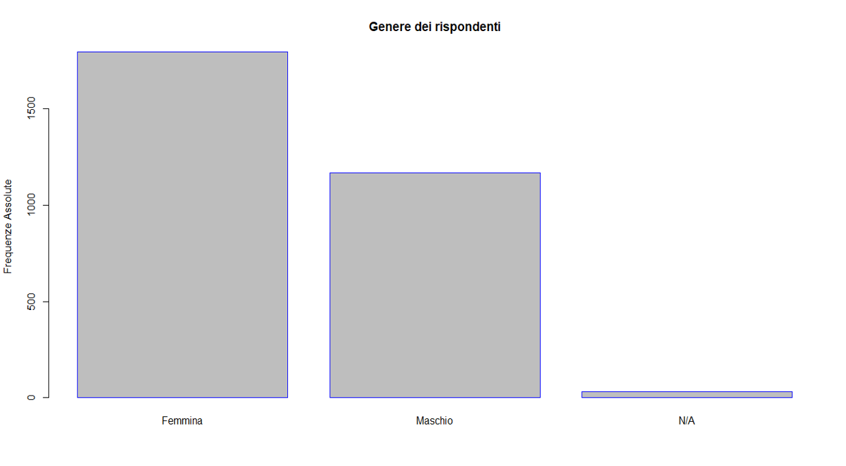
BAR CHART ⮚Useful for qualitative characters and to highlight the absolute frequencies of each variable.
X<-table(sesso) barplot(x, main="Genere dei rispondenti", border="blue", ylab="Frequenze Assolute")
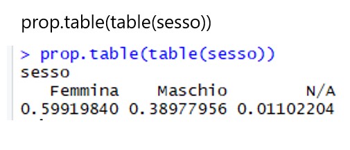
BAR CHART: Calculate relative frequencies
|

This course presents the concept of RStudio Software. We will learn the history the computing environment Analysis Techniques Community, how to install it, and we will explore RStudio Creating a Project Notebook.
Related training material