|
Principal component analysis (PCA)
Introduction
Introduction Click to read 
Principal component analysis (PCA) is a statistical multivariate analysis technique for dimension reduction. In practice it is used when there are many correlated variables within a dataset, in order to reduce their number, losing the smallest possible amount of information.
PCA has precisely the aim to maximize variance, calculating the weight to be attributed to each starting variable in order to be able to concentrate them in one or more new variables (called principal components) which will be a linear combination of the starting variables.
PCA requirements
PCA requierements Click to read
Variable Analysis
|
To understand whether it makes sense to conduct principal component analysis, it is important to analyze the variables to be used in order to have clear some of their characteristics. Specifically, the variables must meet the following requirements:
|
 |
- Variables must be Quantitative
|
PCA is valid only when the variables are numeric. In case of different units of measurement, you need to standardize the variables before proceeding. However, in some cases it is also used for “Likert scale” variables and for “binary variables”. Although numerically the results are very similar to each other, in these cases it would be preferable to use alternative methods.
|
 |
- There must be a linear correlation between variables
The first thing to do when doing a PCA is to calculate the variance/covariance matrix or Pearson correlation matrix. PCA in fact is a technique that can be used when the assumptions of the Pearson linear correlation coefficient are respected. Pearson's correlation coefficients inform you about the direction and intensity of the linear relationship between phenomena. To interpret it, remember that the closer the coefficient is to zero, the weaker the relationship will be, the closer it gets to -1 or +1, the stronger the relationship will be. In PCA, acceptable values for this indicator are R>0.3 or R<-0.3. If a variable had correlation coefficients very close to 0 with all the other variables, then that variable should not be included in the PCA. Forcing that variable to merge with others will result in a very high loss of information and this is something that is generally better to avoid.
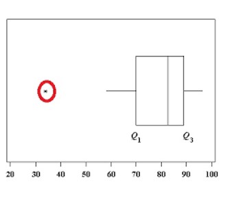
- Lack of outliers
|
As with all variance-based analyses, single outliers can affect the results above all if they are very large and if the sample size is small.
To this end, It is useful to create boxplots or scatter plots, from which it is possible to deduce linear relationships between pairs of variables.
|
 |
Quite large sample size
|
There is no univocal threshold value, but generally speaking it is advisable to have at least 5-10 statistical units for each variable you want to include in the PCA. For example, if you want to try to summarize 10 variables with new components, it would be advisable to have a sample of at least 150 observations.
|
 |
How to conduct PCA
How to conduct PCA Click to read
- Sample adequacy
After verifying the dataset requirements, checking that the variables have the right characteristics to be able to conduct the principal component analysis, here are the different steps to conduct it:
Check the adequacy of the sample through:
- The Kaiser-Meyer-Olkin test, (KMO), which establishes whether the variables considered are actually consistent for the use of a principal component analysis. This index can take values between 0 and 1 and, in order for a principal component analysis to make sense, it must have a value at least greater than 0.5.
This index can be calculated as a whole for all the variables included in the PCA.
-Bartlett's sphericity test: it is a hypothesis test that has as null hypothesis that the correlation matrix coincides with the identity matrix. If so, it would make no sense to perform a PCA as it would mean that the variables are not linearly related to each other at all. As with all hypothesis tests, the value to stop at in order to decide whether to reject the null hypothesis or not is the p-value. In this case, for the model to be considered valid, a p-value lower than 0.05 must be achieved. In this case, in fact, the null hypothesis can be rejected with a significance level of 5%.
Principal components’ extraction Click to read
The crucial part of PCA is to establish the adequate number of factors that can best represent the starting variables.
To better understand this concept, imagine that your dataset is a city you don't know, and each major component is a street in this city. If you wanted to get to know this city, how many streets would you visit? You would probably start from the central street (the first main component) and then explore other streets. How many though?
In order to say that you know a city well enough, the number of streets to visit varies according to the size of the city and how similar or different the streets are, obviously. Similarly, the number of components to extract depends on how many variables you choose to include in your principal component analysis and how similar they are to each other. In fact, the more correlated they are, the lower the number of principal components necessary to obtain a good knowledge of the starting variables. Conversely, the less they are correlated, the greater the number of principal components to be extracted in order to have accurate information about the dataset.
The criteria used for choosing the number of components are essentially two: eigenvalues greater than 1 and parallel analysis.
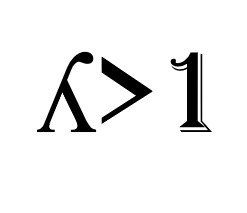
- Eigenvalues greater than 1
|
According to this rule, we choose those components with an eigenvalue greater than 1.
The eigenvalue is a number that returns the variance explained by the component: since initially the variance explained by each individual variable is equal to 1, it would not make sense to take a component (which is a combination of variables) with a variance of less than 1.
A high eigenvalue corresponds to a greater variance and software such as SPSS or R return this table with decreasing values; therefore, the first one will always be associated with the most important factor.
|
 |
- Proportion of Explained Variance
Following this criterion, the components to be extracted must ensure that at least 70% of the overall variability of the starting variables is not lost. Furthermore, each single component to be extracted should bring a significant increase in the overall variance (for example, at least 5% or 10% more of explained variability).
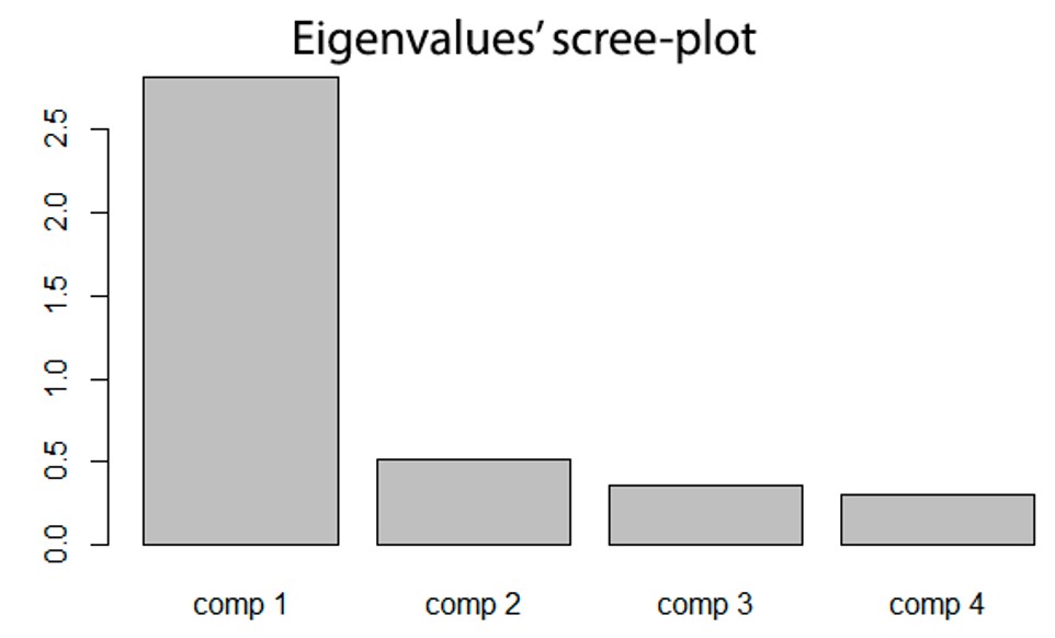
- Scree Plot
|
This method is based on a graph in which the values of the eigenvalues are shown on the vertical axis and all the possible components to be extracted on the horizontal axis (which will therefore be equal in number to the starting variables). By joining the points you will obtain a broken line which in some parts will have a concave shape and in others a convex one.
|
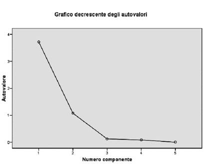 |
As you can see from the graph, the components are listed on the x axis, whereas the eigenvalues are on the y axis. When the curve on this graph makes an "elbow" it's time to draw a line, and take into consideration only the factors which are above.
From the graph above, for example, you can see that the number of points above the elbow is 2.
The final part of PCA consists in giving a name to the individual main components found.
PCA with R
PCA with R Click to read
With statistical software (such as SPSS, Jamovi and R) PCA is a very simple operation. A few clicks are enough to be able to obtain an output to be interpreted. There is therefore no software that is preferable to the others as it is a widely used technique and all statistical programs allow it to be performed easily and without having to carry out any hand calculation. However in this module we will show how to conduct PCA with the R software.
The whole process to implement PCA on R will be represented in the power point attached to this module, namely:
- Carrying out all the steps that are based on matrix, geometric and statistical proofs;
- Through the PCA direct command of the FactoMineR package.
In this module we will just present the FactoMineR package.
FactoMineR is able to carry out principal components analysis by reducing the dimensionality of the multivariate data to two or three, which can thus be displayed graphically with a minimum loss of information and this can be done using a single command, that is PCA, we will insert the matrix object of analysis between parentheses
X <- as.matrix(DATASET)
library(FactoMineR)
res.pca = PCA(DATASET)
With the summary command we can see the importance of the components in terms of standard deviation, proportion of explained variance and cumulative explained variance, both for individuals and for variables.
summary(res.pca)
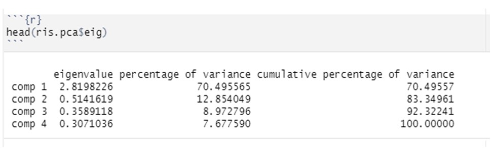
With the head command
head(ris.pca$eig)
instead, you can calculate the importance of the eigenvalues. The command, in fact, will give us the values of the eigenvalues, the percentage of the explained variance and the cumulative explained variance for each variable.
Example of what we will see on R
Finally, in order to be able to draw the scree-plot of the eigenvalues, we will insert the object of analysis between parentheses
barplot(res.pca$eig[,1], main="Eigenvalues’ scree-plot")
With the Main command we’ll indicate the title of the graph.
Example of what we will see on R
Another useful package for PCA (we won't cover it in this module though) is factoextra, which provides some easy-to-use functions to extract and visualize the results we get from multivariate analyses, including PCA (principal component analysis), CA (simple correspondence analysis), MCA (multiple correspondence analysis), MFA (multiple factor analysis), HMFA (hierarchical multiple factor analysis).
|
 Play Audio