|
Generalized linear models: ANOVA
Introduction
Introduction Click to read 
The GLM techniques presented here in the form of Analysis Of Variance (ANOVA) allow for responding to potentially interesting questions. Some examples:
- Are male and female workers in a region making the same mean annual wage?
- Do the students of a course following different teaching methods getting the same mean grade?
- Is the mean weekly consumption of certain medicine different across age groups and/or gender?
One-factor ANOVA is fine for questions 1 and 2, while question 3 requires of two-factor ANOVA. Our goal is to test for the effect of an independent variable (factor) classified into k several categories (levels) on a numerical dependent variable (response variable), and it bases on decomposing total sample variability. We can approach this problem as a statistical hypothesis test of a null hypothesis (H0; our default) versus and alternative (H1; an alternative worldview). The test is formulated in terms of the population means of the response variable across the levels of our factor(s).

The assumptions required to conduct the ANOVA test are:
- Normal populations: the distribution of the response variable on each and every level should be normal
- Equality of variances: the variances of the response variable across levels must be the same
- Independent simples: the sample data on each level of the factor is nor correlated with the other sample data (collected from the other levels)
One way ANOVA
The procedure Click to read
The ANOVA procedure with one factor bases on the following equation:
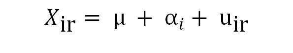
where xir is the value of our response variable for individual r at category (level) i. We assume that this value is the sum of three effects:
- A grand mean value (μ), common to all the individuals and levels
- A shift (αi) that captures the mean influence of belonging to level i
- A residual (uir) , which accounts for random, uncontrolled variations. This residual is assumed to distribute normally with zero mean
The ANOVA test is equivalent to test if the αi terms are identical across the k levels. If not, there will be significant differences in the means.
We take sample data on X and decompose its variability (dispersion around the sample means) into two parts:
- The within group (SSW) accounts for the internal variability.
- The between variability (SSB) accounts for the differences between each group sample mean and the grand mean.
The total variability (SST) is just the sum of SSW+SSB. If SSB is much larger than SSW, it indicates than there are significant differences in the group means. So, there will be significan differences in the means across the levels of the factor.
In order to compare the relative weight of SSB and SSW on the total variability, we scale them dividing by the number of degrees of freedom, producing the values MSB and MSW respectively.

If the assumptions required hold, the statistic (d) computed as MSB∕MSW distributes as a F-model. This statistic allows for making a decision about the test: the higher its value, the larger (relatively) is the between part when compared with the within variability.
An example Click to read
As an illustrative example, suppose want to test if the design of the packages on which a specific brand of milk is sold, has any influence on the sales. With this objective, we take a sample of 12 stores with similar characteristics and, settign the same price for the milk, we randomly assign one type of packaging (1, 2 or 3). Then we get the sample data of our response varaible “Sales”, which measures how many thousands milk bottles were sold in one month, as depicted below:
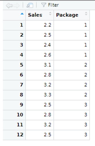
Our sample data shown above is contained in a R file, which we can open by going here (we are calling this data file “Milk”):

We want to test if there are statistically significant differences in the mean sales, depending on the designg of the package. We are applying ANOVA with R, which requires installing specific packages:

In order to apply ANOVA, we first need to make sure that the assumptions required actually hold, so we run the following pieces of code:
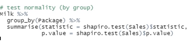
These lines first indicated the dataset that is considered (“Milk”), then group the data by the levels of the factor (“Package”) and finally runs a Spahiro normality test on our response variable (“Sales”) across groups:
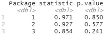
The high p-values of this normality test for all the levels allow us to work under the required assumption of normality. Additionally, we also assume to have equal variances, which leads us to run a Barlett test of homogenous variances as shown below:
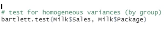
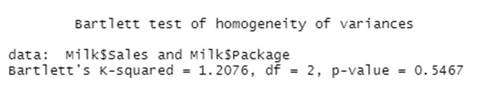
The p-value displayed below suggests that this assumption is hihgly realistic:
Given that the necessary assumption seem to hold, we conduct the ANOVA methodology by running the following code lines:
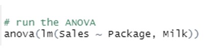
Which produces the following output:
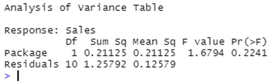
The results of the ANOVA test indicates that the differnt designs of the packages seem not to impact on the mean sales: the part of variability explained by the different levels of the factor “Package” (between variability) is not significantly larger than the residual part (within variations). As a consecuence, the p-value associated to this test is high and telss us that there are not reasons to reject the null hypothesis of equal mean sales across designs.
Two factor ANOVA
The procedure Click to read An example Click to read
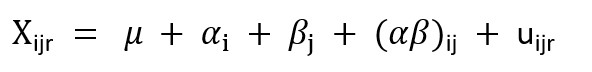
We are going to illustrate empirically of the two-factor ANOVA works, assuming that we have the following problem: A health centre wants to analyze the potential influence of age and sex on the use of a medicine. A sample survey is conducted for this purpose and users were grouped by age into four categories (children, teenagers, adults, seniors) and gender. A sample of 24 individuals was drawn, independently selecting 3 individuals by gender and age group. The response variable is the monthly consumption of this medicine (in €), and we have the followng dataset:
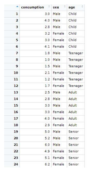
Again, the sample data shown above (contained in a R file called “medicine), can be loaded in Rstudio by going here:

Now, we are applying a two-factor (age and gender) ANOVA with R, which requires installing and loading specific packages:
In order to apply ANOVA, we first test if the assumptions required actually hold, by running normality and equal-variances test. Normality tests (across all the age groups and the two genders) are conducted by running:
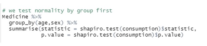
We first indicate the dataset that is considered (“Medicine”), then group the data by the levels of the tow factors considered in our anlaysis (“age” and “sex”) and finally runs a Spahiro normality test on variable “consumption” across all the groups:
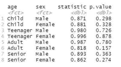
Note that now, when referring to the levels of the two factors, we need to consider all pairs of possible categories between them. Agian we find high p-values for this normality test in all the cases, which allow us to work under the required assumption of normality. Moreover, homogenous variances are required as well, and in this case this assumption is tested by conducting a Levene test as:

The p-value found indicates that we do not have empirical evidence in the sample against this assumption either:

Since the assumptions required to conduct a two-factor ANOVA process seem to hold, we do it by running the following code lines:
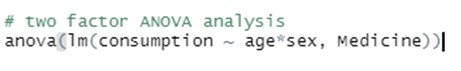
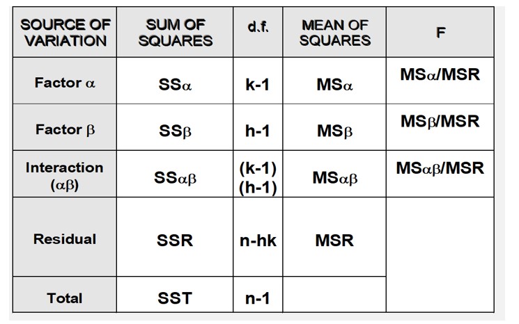
The output of the analysis comes in the form of the following multiple ANOVA table:
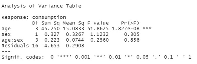
The results of this two-factor ANOVA provides very useful information that allows to give a data-based response to our research question. The tests conducted indicates that the mean values of the consumption of the medicine are significantly different across the four levels of the factor “age” (note that is the only case when we have a low p-value, which leds to reject the null hypothesis of equal means). However, neither we find significant differences in the mean consumption by gender or across the interactions between age-group and gender.
|
 Play Audio